Testing a Thermal Fluid Loop with Simulation and Embedded Control
A Python simulation, a shared C controller, and a browser tool for exploring how a fluid loop responds to faults.
Virtual Thermal Fluid Lab is my software test bench for exploring how fluid flow, heat transfer, and embedded control interact. I can run a healthy loop, introduce a restriction or a sensor fault, and follow the resulting behavior from the controller’s inputs through to the simulated temperatures.
The project brings together three tools: a Python plant model, an actual C controller executable, and a browser replay. Each has a clear job, and the recorded interfaces make it possible to investigate the whole experiment without needing a physical rig for every software change.
Project scope
The lab includes an atmospheric tank benchmark and a closed thermal circulation loop. Its software covers conservation equations, pump and valve dynamics, flow control, protective trips, sensor and transport faults, and reproducible experiment records. A static visualization tool makes those records easy to explore and compare.
I scoped the model around questions the software can answer clearly: how does added resistance affect flow, can the controller recover its target, and what happens when a cooling request cannot remove heat? Coefficients are assumed, and the reported temperatures and flows are simulation outputs. Physical experiments are a separate next step.
How the software fits together
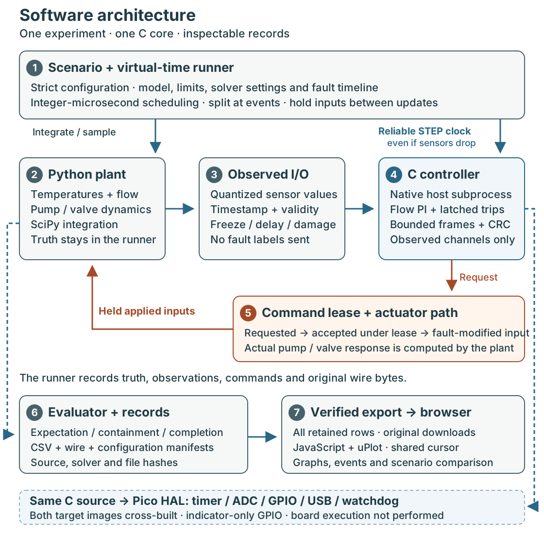
Configure and simulate. A scenario specifies the model, controller limits, event timeline, and solver settings. Strict validation catches ambiguous or invalid inputs before a run starts. The Python runner schedules events using integer microseconds, splits integration at changes, and holds applied commands between updates. SciPy integrates the plant’s temperatures and actuator dynamics.
Observe and control. An adapter turns plant outputs into sensor frames with timestamps and validity information. It can freeze values or delay, drop, and damage transport. The portable C11 core receives observed I/O, never plant truth or fault labels. It combines flow PI control, saturation and anti-windup, and a latched supervisor. A separate, reliable STEP frame advances controller time even when sensor frames disappear.
Apply and record. The native C subprocess exchanges bounded, checksummed ASCII frames with Python. Its requested commands pass through a lease and actuator-fault path before reaching the plant. This preserves the difference between requested, accepted, applied, and actual behavior. The evaluator reports expectation, containment, and completion separately; CSVs, wire captures, and manifests retain configuration, source, solver, and file hashes.
Inspect and reuse. The exporter verifies those hashes and preserves every retained row. JavaScript and uPlot provide synchronized graphs, playback, event selection, absolute-time comparison, and raw downloads. The browser reads completed experiments; it does not run the simulation. The same C core also compiles into Pico targets with timer, ADC, GPIO, USB, and watchdog wrappers. Both images build; execution on a board remains unperformed.
How the thermal simulation works
The original tank provides an approachable benchmark: inflow minus gravity drainage changes its level. Analytic fill, drain, lag, and boundary cases check the implementation.
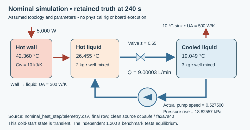
The thermal model adds three energy stores: a heated wall, a mixed hot liquid inventory, and a mixed cooled inventory. Circulation exchanges liquid between the inventories, while the cooled side rejects heat to a fixed-temperature sink. Density, mass, and heat capacity are constant.
Cw dTw/dt = P - UAh (Tw - Th)
Ch dTh/dt = UAh (Tw - Th) + rho Q cp (Tc - Th)
Cc dTc/dt = rho Q cp (Th - Tc) - UAc (Tc - Ts)
Every right-hand term is power in watts. Adding the equations cancels internal exchange and circulation, leaving heat input minus rejected heat. This energy-balance reasoning gives an independent way to check the model.
Flow comes from the intersection of an assumed pump curve and loop resistance:
Pump pressure rise: p0 x² - Kp Q²
Loop pressure drop: (Kpipe + Kvalve/z²) Q², for z > 0
Here x is normalized pump speed and z is valve opening. Kvalve has units Pa·s²/m⁶; closure has an explicit zero-flow branch. Pump speed and valve opening respond with first-order lags.
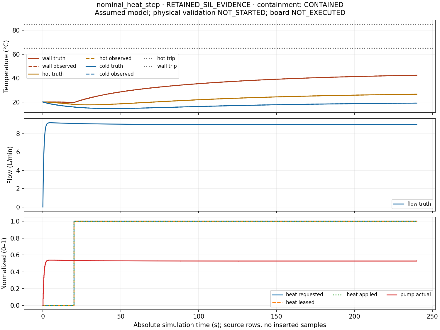
At 9 L/min and 5,000 W, independently calculated equilibrium temperatures are about 20 °C cooled liquid, 27.97 °C hot liquid, and 44.64 °C wall. The equilibrium test runs for 1,200 simulated seconds; the 240-second nominal example is still warming up.
Example: recovering flow after a restriction
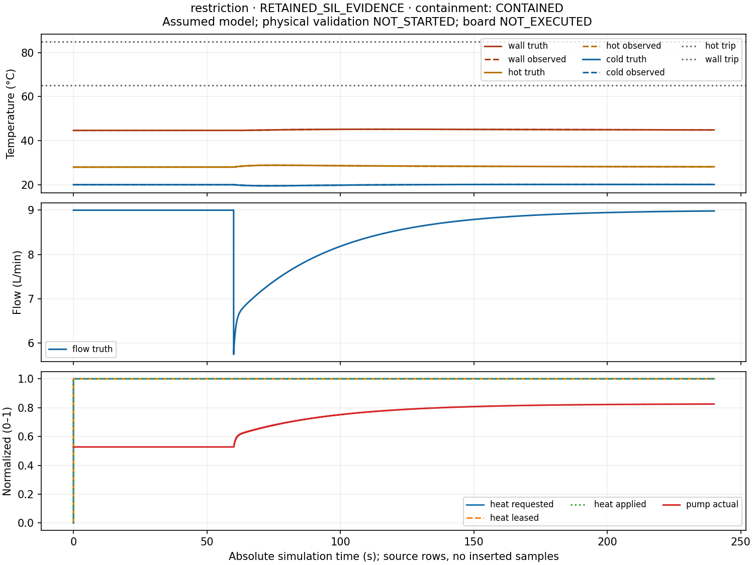
At 60 seconds, the restriction scenario quadruples pipe resistance while leaving the valve opening at 0.65. Flow immediately falls from 9.00 to 5.74 L/min at the existing pump speed. The controller sees the flow error and increases its pump request; the plant’s lag determines how quickly actual speed follows.
By 240 seconds, actual pump speed has risen from about 0.527 to 0.825, and flow has recovered to 8.98 L/min. The run completes without a trip. This example connects the hydraulic operating point, the PI response, and the thermal consequence in one trace.
Example: inspecting temperature and heater faults
The frozen-temperature scenario keeps plausible primary readings arriving with fresh timestamps while true temperatures rise after loss of heat rejection. Freshness alone cannot detect that problem. A separately emulated temperature switch provides the discriminating signal and trips the controller at 343.9 seconds.
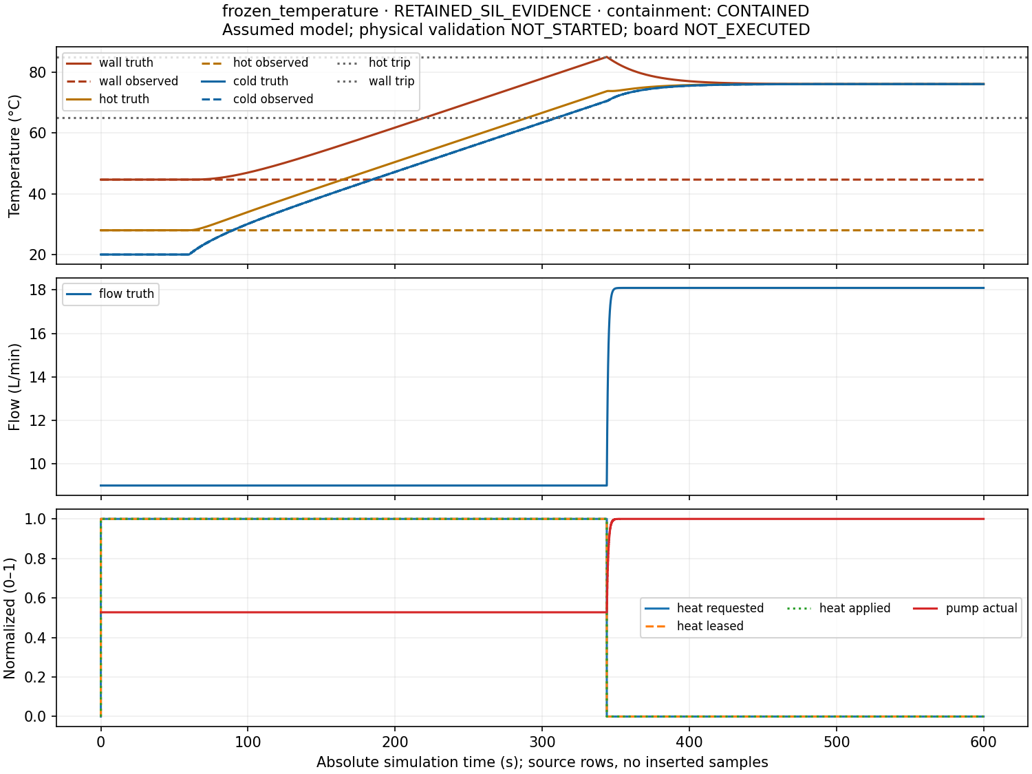
The frozen and biased cases remain below a conservative 85.059 °C bound, excluding integration error, against the chosen 86 °C criterion. Their heat-off and maximum-circulation requests take effect under the declared actuator assumptions.
The stuck-heater case explores a different outcome: heating remains at 5,000 W and sink conductance becomes zero. The energy balance predicts continuing heat accumulation. The controller trips at 346.6 seconds, but applied heating continues until the wall reaches the 95 °C model boundary at 466.299590 seconds.
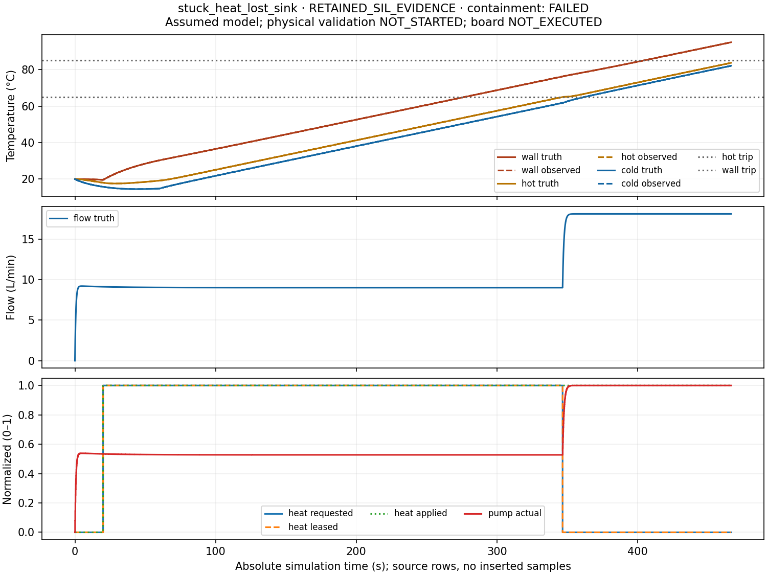
The expected-hazard test passes, containment is FAILED, and the requested 1,200-second horizon is incomplete. Keeping those judgments separate is an essential feature of the software.
Explore the results
The interactive replay puts temperatures, flow, commands, actuator state, and events on one cursor. Try the restriction case, then compare frozen readings with plant truth. Raw downloads let any plotted value be followed back to its original record.
Verification passed 135 unit tests, ten thermal benchmarks, seven preserved Python tank scenarios, all 17 thermal and seven C tank cases, and a byte-identical nominal repeat. All 36 refinement runs passed. Independent equations check heating, cooling, equilibrium, pressure, and boundaries; solver refinement is assessed separately from controller timing. Windows/MSVC, Linux/GCC, sanitizers, and Pico cross-build CI passed for the release.
The selected 240-second demo took 8.43 wall seconds on the Windows workstation. Its observed process peaks met the chosen laptop budget, with monitoring limits documented; this is not a hard-real-time claim. The source and release include reproduction commands and the full evidence.
Physical validation remains NOT_STARTED. The lumped thermal model omits fluid travel-time delays, local gradients, phase change, and pump dissipation. The next experiment is an indicator-only Pico capture of acquisition, arming, latching, reconnects, and timing, followed by measured water-loop experiments with separate holdout runs.